IMAGE AS FUNCTION 🎞→().
- chalapathinagavarma bhupathiraju

- May 8, 2020
- 3 min read
Updated: Jun 2, 2020
In the previous blog (alphabets of computer vision) introduce computer vision. Let's dive deeper 🙂🙂.
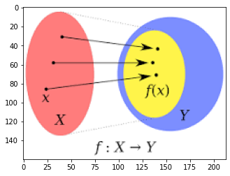
I am saying an image is a function. You may think I am a fool😛😛 , but the images we use in our daily life have some intensity which means every pixel in the image has some intensity.

Let us take a black and white image. This black and white image contains intensity from 0 to 255. You may ask why only from 0 to 255. It depends on bit depth. If we are having 1bit there are 8 bytes so 255 is highest.255 represents a white and 0 represents a black, in between represents gray.

If we take two-dimensional images it is having x and y-direction. Mathematically image is
F(X, Y).if we want pixel 3 from the x-axis and 2 from the y-axis then it will be F(3,2).
The color image contains 3 channels that are R, G, B channels so the function will be
F(X, Y) = [R(X,Y),G(X,Y),B(X,Y)]
Let us look at how to load images and display images in python.
import numpy as np
import matplotlib.pyplot as plt
import cv2
image = cv2.imread("/content/image as function.png")
#The open cv reads images in BGR so we have to convert into RGB
image = cv2.cvtColor(image,cv2.COLOR_BGR2RGB)
plt.imshow(image)
# if we want  22 row and 120 coloumn then
print(image[22,120,:])
OUTPUT:
[255 255 255]
cropping an image
In our daily life, we crop so may images. This time we do with python, Consider the above figure in that let us thing we only need the pink part of the image. the pink part of the image is the range between 0 to 140 in the x-direction and 0 to 74 in the y-direction. it can be done in simple slicing
croped_image = image[0:140,0:74,:]

Merging of the images:
If we are thinking of an image as the function we know we can add two functions then we can add two images.
we can add two images as below
import numpy as np
import matplotlib.pyplot as plt
import cv2
image1 = cv2.imread("/content/orginalmatlab.png")
image2 = cv2.imread("/content/tensorflow.png")
image1 = cv2.resize(image1,(281,179))
image1 = cv2.cvtColor(image1,cv2.COLOR_BGR2RGB)
image2 = cv2.cvtColor(image2,cv2.COLOR_BGR2RGB)
image3 = image1 + image2
plt.subplot(131)
plt.imshow(image1)
plt.xticks([])
plt.yticks([])
plt.subplot(132)
plt.imshow(image2)
plt.xticks([])
plt.yticks([])
plt.subplot(133)
plt.imshow(image3)
plt.xticks([])
plt.yticks([])
output:

In this output there a pitfall that when bright areas get added resulted in the dark.because
let us think if we are adding pixels 255 and 10 it will result in 10(i.e (265)%255) as the type of images is uint8. In order to avoid this problem, OpenCV provides a function add. Let us what will happen if we did that.
import numpy as np
import matplotlib.pyplot as plt
import cv2
image1 = cv2.imread("/content/orginalmatlab.png")
image2 = cv2.imread("/content/tensorflow.png")
image1 = cv2.resize(image1,(281,179))
image1 = cv2.cvtColor(image1,cv2.COLOR_BGR2RGB)
image2 = cv2.cvtColor(image2,cv2.COLOR_BGR2RGB)
image3 = cv2.add(image1,image2)
plt.subplot(131)
plt.imshow(image1)
plt.xticks([])
plt.yticks([])
plt.subplot(132)
plt.imshow(image2)
plt.xticks([])
plt.yticks([])
plt.subplot(133)
plt.imshow(image3)
plt.xticks([])
plt.yticks([])
output:

know it is clear.
Noise
Noise is just like another function that is combined with the original function to give a new function.
I(X, Y) = F(X,Y) + noise(X,Y)
Types of noise:
Gaussian noise
Salt pepper noise
Salt pepper noise
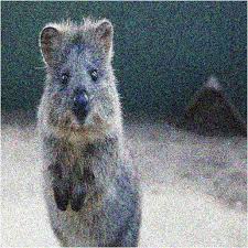
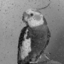
Gaussian noise Impulse noise Salt pepper noise
Salt pepper noise:
It takes the original picture and sprinkles white spots and occasional dark spots.
Impulse noise:
It adds a random occurrence of white pixels to the original image
Gaussian noise:
Gaussian noise is generated from the normal distribution. This noise is added to the original image.
Gaussian distribution is very important in image processing. Gaussian noise is generated from the gaussian distribution. Gaussian distribution has 0 mean and 1 variance. we can generate Gaussian distribution in python using np.random.randn().we can change the variance of the distribution by multiplying with a wanted variance that is sigma. As the variance increases the spreading of data will increase Let us see with code and visualization.
import numpy as np
import matplotlib.pyplot as plt
import cv2
original_noise =  np.random.randn(200,200)
noise1 = original_noise * 2
noise2 = original_noise * 8
noise3 = original_noise * 32
noise4 = original_noise * 64
plt.subplot(221)
plt.imshow(noise1,cmap = 'gray')
plt.xticks([])
plt.yticks([])
plt.title("sigma = 2")
plt.subplot(222)
plt.imshow(noise2,cmap = 'gray')
plt.xticks([])
plt.yticks([])
plt.title("sigma = 8")
plt.subplot(223)
plt.imshow(noise3,cmap = 'gray')
plt.xticks([])
plt.yticks([])
plt.title("sigma = 32")
plt.subplot(224)
plt.imshow(noise4,cmap = 'gray')
plt.xticks([])
plt.yticks([])
plt.title("sigma = 64")
Adding noise to images using OpenCV
python code for adding noise to images
before going to see the code let me give you some cv2 functions
cv2.randu() randomly generates a uniform distribution in a given range which means it will form a matrix having only one value in it.
Ex:[[1,1],[1,1]].
cv2.threshold() takes a image,lower_bound,and upper_bond.If an intensity in the image between lower and upper bound it will give 255 else it will give values to zero.
Ex: image = [[1,100],[220,0]],lower_bound = 100,upper_bound = 250 then It will return
[[0 250],[250, 0]]
import numpy as np
import matplotlib.pyplot as plt
import cv2
image1 = cv2.imread("/content/tensorflow.png",cv2.IMREAD_GRAYSCALE)
u = np.zeros(image1.shape)

uniform_noise = cv2.randu(u,0,255).astype(np.uint8)

_,impulse_noise = cv2.threshold(uniform_noise,250,255,cv2.THRESH_BINARY)
impulse_noise = impulse_noise.astype(np.uint8)
normal_noise = np.random.randn(image1.shape[0],image1.shape[1]).astype(np.uint8)
noise1 = image1
noise2 = cv2.add(image1,uniform_noise)
noise3 = cv2.add(image1,impulse_noise)
noise4 = cv2.add(image1,normal_noise)
plt.subplot(221)
plt.imshow(noise1,cmap = 'gray')
plt.xticks([])
plt.yticks([])
plt.title("original")
plt.subplot(222)
plt.imshow(noise2,cmap = 'gray')
plt.xticks([])
plt.yticks([])
plt.title("uniform")
plt.subplot(223)
plt.imshow(noise3,cmap = 'gray')
plt.xticks([])
plt.yticks([])
plt.title("impulse")
plt.subplot(224)
plt.imshow(noise4,cmap = 'gray')
plt.xticks([])
plt.yticks([])
plt.title("gaussian ")
In the next blog, we will see about filters😉😉😉 . see you there


Comments